Direct information from a multiple sequence alignment

In this example, we compute coupling strengths between residues of the CRISPR-Cas9 protein amino acid sequence from multiple sequence alignment data. We demonstrate that a statistic called direct information [1] computed from these couplings is predictive of contacts in observed 3D conformations of the sequence.

We start by loading the necessary packages and functions. We collect and parse MSA data from the Pfam database using the parse_pfam function in this script. The function downloads the full current release of the Pfam database, creates a local directory structure with the MSA data for each family and any cross-references from sequences in each family to structures in the Protein Data Bank, then returns pandas DataFrames that detail information about the MSAs and PDB cross-references.

The MSA and PDB cross-reference data for the protein family/MSA with Pfam accession code PFXXXXX are stored in files msa.npy and pdb_refs.npy (if cross-references are found) in the Pfam-A.full/PFXXXXX subdirectory of data_dir defined below.

import matplotlib.pyplot as plt
from matplotlib import patches
import numpy as np
import pandas as pd
from scipy.spatial import distance_matrix
import fem, sys, os, time, Bio.PDB, nglview, warnings
pdb_list = Bio.PDB.PDBList()
pdb_parser = Bio.PDB.PDBParser()
data_dir = '../../../data/msa'
sys.path.append(data_dir)
from parse_pfam import parse_pfam
from Bio import BiopythonWarning
warnings.simplefilter('ignore', BiopythonWarning)
%matplotlib inline

Next, we get pandas DataFrames pfam and pdb_refs detailing information for all protein families in the Pfam database and references from MSA sequences to PDB structures.

pfam, pdb_refs = parse_pfam(data_dir)
print 'total MSAs: %i, total PDB refs: %i' % (pfam.shape[0], pdb_refs.shape[0])

total MSAs: 16479, total PDB refs: 207746

Each row in pfam contains information about a single MSA. The columns of pfam are res: the number of residues in each sequence of the alignment, seq: the number of sequences in the alignment. Now let’s add a column size=res*seq and sort by that column to see which families contain the most data.

pfam['size'] = pfam['res'] * pfam['seq']
pfam.sort_values(by='size', ascending=False, inplace=True)
pfam.head()

	res	seq	pdb_refs	size
PF00005	2386	369723	407	882159078
PF00069	3194	236455	3910	755237270
PF07690	3427	214283	23	734347841
PF00067	4853	85020	768	412602060
PF00501	3767	87704	145	330380968

Each row in the PDB references table pdb_refs contains information about a cross-reference between a protein family sequence in the Pfam database and a protein structure in the PDB database. The columns of the table are seq: the index (starting at 0) of a sequence in the protein family, uniprot_id: the ID of the sequence in the UniProtKB database, uniprot_start/uniprot_end: the start and end residue positions of the UniProtKB sequence that appears in the MSA, pdb_id: the PDB ID, chain: the PDB protein structure chain, pdb_start/pdb_end: the start and end residue positions of the PDB sequence that appears in the MSA. Let’s create a column res that contains the length of the sequence and sort by that column.

pdb_refs['res'] = pdb_refs['pdb_end'] - pdb_refs['pdb_start'] + 1
pdb_refs.sort_values(by='res', ascending=False, inplace=True)
pdb_refs.head()

	seq	uniprot_id	uniprot_start	uniprot_end	pdb_id	chain	pdb_start	pdb_end	res
PF11894	578	NU205_HUMAN	14	1684	5IJN	J	14	1684	1671
PF11894	578	NU205_HUMAN	14	1684	5IJN	P	14	1684	1671
PF11894	578	NU205_HUMAN	14	1684	5IJN	D	14	1684	1671
PF11894	578	NU205_HUMAN	14	1684	5IJN	V	14	1684	1671
PF02463	2434	SMC1_YEAST	3	1213	1W1W	C	3	1213	1211

We’ll examine the particular protein family with Pfam accesion code PF16592. This protein family corresponds to the REC lobe of CRISPR-associated endonuclease Cas9. The REC lobe and the NUC lobe of Cas9 fold to present a positively charged groove at their interface which accommodates the negatively charged sgRNA: target DNA heteroduplex. [2] We’ll isolate the family of interest from the pfam DataFrame in the fam variable.

# Cas 9 family accesion code
ac = 'PF16592'
# store the family of interest in the 'fam' variable
fam = pfam.loc[ac]
print 'size rank: %i of %i' % (pfam['size'].rank(ascending=False)[fam.name].astype(int), pfam.shape[0])

# local directory containing data for this MSA
fam_dir = os.path.join(data_dir, 'Pfam-A.full', fam.name)
# the residue symbols array that is the MSA
msa = np.load(os.path.join(fam_dir, 'msa.npy'))

# determine which residues are the same across all sequences, excluding gaps
aa = np.array([np.unique(s) for s in msa])
one_aa = np.array([len(a) == 1 for a in aa])
two_aa = np.array([len(a) == 2 for a in aa])
missing_aa_res = np.array(['-' in a for a in aa])
conserved_residues = one_aa | (two_aa & missing_aa_res)

# the number of unique amino acids (or gap symbol) that appear at each residue
m = np.array([len(a) for a in aa])
m = m[~conserved_residues]
n_residues = m.shape[0]

pfam[pfam.index == ac]

size rank: 7142 of 16479

	res	seq	pdb_refs	size
PF16592	1079	146	21	157534

One can classify a residue from the perspective of the MSA as a conserved residue, meaning that in every sequence of the MSA, either a gap or the same amino acid is observed. One can also classify a residue from the perspective of the sequence as a gap, i.e. an insertion that Pfam’s aligning algorithm made in the sequence in order to compare like residues across sequences. Therefore, each sequence-residue symbol is in one of four classes according to whether it is a conserved residue or not and where it is a gap or not. We color code each sequence-residue symbol for the MSA of interest.

code = np.zeros(msa.shape, dtype=int)
code[conserved_residues] = 2
for j, s in enumerate(msa.T):
    code[s == '-', j] += 1

fig, ax = plt.subplots(1, 1, figsize=(16, 4))
ax.set_ylabel('sequence')
ax.set_xlabel('residue')
cmap = plt.cm.get_cmap('plasma', 4)
ax.matshow(code.T, aspect='auto', cmap=cmap)
labels = ['active', 'alignment gap', 'conserved residue', 'alignment gap and conserved residue']
handles = [patches.Patch(color=cmap(i), label=labels[i]) for i in range(4)]
plt.legend(handles=handles, ncol=4)
plt.show()

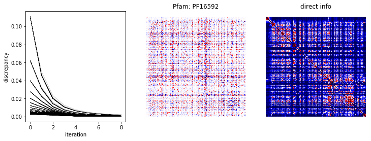
Now, we compute the residue coupling strengths and the direct information from the MSA. The MSA is a set of sequences \(\text{MSA}=\{s_1,\ldots,s_n\}\) and each nonconserved residue \(r_i\), \(i=1,\ldots,m\), in the alignment takes

\[m_i = \left|\{a : r_i=a\text{ for some sequence }s=(r_1,\ldots,r_m)\in\text{MSA}\}\right|\]

unique empircal values in the alignment. In the following, let \(M_i=\sum_{\tilde{i}<i}m_{\tilde{i}}\) for \(i=1,\ldots,m\) and let \(e_i\) denote the \(i^{th}\) canonical basis vector of the shape implied by context.

We use FEM to infer the couplings \(W\) assuming that the probability of residue \(r_i\) being amino acid \(a_k\) for any sequence with one-hot encoding \(\sigma\) is given by

\[p(r_i=a_k~|~\{r_1,\ldots,r_n\}\setminus \{r_i\})={\exp e_{M_i+k}^TW\sigma\over\sum_{j=1}^{m_i}\exp e_{M_i+j}^TW\sigma},\quad i=1,\ldots,m,~k=1,\ldots,m_i.\]

Specifically, we call fem.discrete.fit.model.fit(msa[~conserved_residues]) below, where msa is an array of symbols with each row storing residue data and each column storing sequence data, to return \(W\) and the running discrepancies from the fit.

After computing \(W\), we compute the direct information for each pair of nonconserved residues. The direct information of residues \(r_i\) and \(r_j\) is

\[DI(r_i, r_j)=\sum_{k_1=1}^{m_{i_1}}\sum_{k_2=1}^{m_{i_2}} p(r_{i_1}=a_{k_1}, r_{i_2}=a_{k_2}) \ln {p(r_{i_1}=a_{k_1}, r_{i_2}=a_{k_2}) \over p(r_{i_1}=a_{k_1})~p(r_{i_2}=a_{k_2})}\]

where the joint and marginal probablities are computed over subsequences containing only residues \(r_i\) and \(r_j\):

\[p(r_{i_1}=a_{k_1}, r_{i_2}=a_{k_2})={\exp e_{M_{i_1}+k_1}^TWe_{M_{i_2}+k_2} \over \sum_{j_1=1}^{m_{i_1}}\sum_{j_2=1}^{m_{i_2}}\exp e_{M_{i_1}+j_1}^TWe_{M_{i_2}+j_2}},\]

\[p(r_{i_1}=a_{k_1})={\sum_{k_2=1}^{m_{i_2}} p(r_{i_1}=a_{k_1}, r_{i_2}=a_{k_2}) \over \sum_{k_1=1}^{m_{i_1}}\sum_{k_2=1}^{m_{i_2}}p(r_{i_1}=a_{k_1}, r_{i_2}=a_{k_2})},\]

and \(p(r_{i_2}=a_{k_2})\) is defined similarly.

We plot the running discrepancies from the fit and heat maps of \(W\) and the direct information below.

def direct_information(msa, cache=True):

    w_file = os.path.join(fam_dir, 'w.npy')
    d_file = os.path.join(fam_dir, 'd.npy')
    if cache and os.path.exists(w_file) and os.path.exists(d_file):
        w = np.load(w_file)
        d = np.load(d_file)
    else:
        model = fem.discrete.fit.model()
        start = time.time()
        model.fit(msa[~conserved_residues], iters=10)
        end = time.time()
        print 'fit time: %.02f sec' % (end-start,)
        w = np.hstack(model.w.values())
        d = model.d
        np.save(w_file, w)
        np.save(d_file, d)

    direct_info_file = os.path.join(fam_dir, 'direct_info.npy')
    if cache and os.path.exists(direct_info_file):
        direct_info = np.load(direct_info_file)
    else:
        mm = np.insert(m.cumsum(), 0, 0)
        w_idx = np.vstack((mm[:-1], mm[1:])).T
        direct_info = np.zeros((n_residues, n_residues))
        for i, ii in enumerate(w_idx):
            for j, jj in enumerate(w_idx):
                p = np.exp(w[ii[0]:ii[1], jj[0]:jj[1]])
                pi, pj = p.sum(axis=1), p.sum(axis=0)
                p /= p.sum()
                pi /= pi.sum()
                pj /= pj.sum()
                direct_info[i,j] = (p*np.log(p/np.outer(pi, pj))).sum()
        np.save(direct_info_file, direct_info)

    return direct_info, w, d

direct_info, w, d = direct_information(msa, cache=False)

fig, ax = plt.subplots(1, 3, figsize=(12,4))
for di in d:
    ax[0].plot(di, 'k-', lw=0.1)
ax[0].set_xlabel('iteration')
ax[0].set_ylabel('discrepancy')
scale = 1e-1 * np.abs(w).max()
ax[1].matshow(w, cmap='seismic', vmin=-scale, vmax=scale)
ax[1].set_title('Pfam: %s' % (fam.name,))
scale = 1e-1 * np.abs(direct_info).max()
ax[2].matshow(direct_info, cmap='seismic', vmin=0, vmax=scale)
ax[2].set_title('direct info')
for a in ax[1:]:
    a.axis('off')
plt.show()

fit time: 17.04 sec

Next, we examine the extent to direct information is predictive of residue contacts of the 3D conformations of sequences in the MSA. Several sequences in this family contain cross-references to PDB structures. We’ll isolate these references from the pdb_refs DataFrame in the refs variable.

refs = pdb_refs[pdb_refs.index.str.contains(fam.name)]
refs.head()

	seq	uniprot_id	uniprot_start	uniprot_end	pdb_id	chain	pdb_start	pdb_end	res
PF16592	70	CAS9_STRP1	181	712	4OO8	A	181	712	532
PF16592	70	CAS9_STRP1	181	712	4CMQ	A	181	712	532
PF16592	70	CAS9_STRP1	181	712	4OO8	D	181	712	532
PF16592	70	CAS9_STRP1	181	712	4ZT0	A	181	712	532
PF16592	70	CAS9_STRP1	181	712	5F9R	B	181	712	532

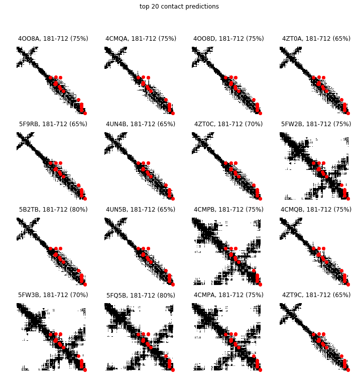
Next, we overlay the greatest direct information pairs on the contact maps of the PDB structures cross-referenced from sequences in the MSA. We indicate the percentage of the greatest direct information pairs that are contacts of the PDB in the title of each subplot. A PDB contact map is a binary image where a pixel value is 1 if the corresponding pair of residues is less than a distance threshold (we use 10 angstroms below) and 0 otherwise.

def contact_map(ref, dist_thresh=10):
    seq = msa[:,ref.seq]
    pdb_file = pdb_list.retrieve_pdb_file(ref.pdb_id, pdir=fam_dir, file_format='pdb')
    chain = pdb_parser.get_structure(ref.pdb_id, pdb_file)[0][ref.chain]
    coords = np.array([a.get_coord() for a in chain.get_atoms()])
    coords = coords[ref.pdb_start-1:ref.pdb_end]
    missing_aa_seq = seq == '-'
    coords = coords[~conserved_residues[~missing_aa_seq]]
    return distance_matrix(coords, coords) < dist_thresh

def predict_contacts(seq, direct_info, top, k=2):
    missing_aa_seq = seq == '-'
    di_idx = np.arange((~conserved_residues).sum())
    di_idx = di_idx[~missing_aa_seq[~conserved_residues]]
    di = direct_info[np.ix_(di_idx, di_idx)]
    mask = np.triu(np.ones(di.shape[0], dtype=bool), k=k)
    thresh = np.sort(np.abs(di)[mask])[-top]
    di[~mask] = 0
    predicted_contacts = np.where(di >= thresh)
    return predicted_contacts

top = 20
max_tp = 0
best_ref = refs.iloc[0]

n_refs = refs.shape[0]
r, c = int(1+(n_refs-1)/4.), 4
w, h = 12, 3*r
fig = plt.figure(figsize=(w,h))
for i in range(refs.shape[0]):
    ref = refs.iloc[i]
    seq = msa[:, ref.seq]
    contacts = contact_map(ref)
    predicted_contacts = predict_contacts(seq, direct_info, top)
    tp = contacts[predicted_contacts].sum()
    if tp > max_tp:
        max_tp = tp
        best_ref = ref

    ax = fig.add_subplot(r, c, i+1)
    ax.matshow(contacts, cmap='Greys', aspect='auto')
    ax.scatter(*predicted_contacts[::-1], c='r')
    ax.set_title('%s%s, %i-%i (%02.0f%%)' % (ref.pdb_id, ref.chain, ref.pdb_start, ref.pdb_end, 100.*tp/float(top)))
    ax.axis('off')

plt.suptitle('top %i contact predictions' % (top,))
plt.show()

Structure exists: '../../../data/msa/Pfam-A.full/PF16592/pdb4oo8.ent'
Structure exists: '../../../data/msa/Pfam-A.full/PF16592/pdb4cmq.ent'
Structure exists: '../../../data/msa/Pfam-A.full/PF16592/pdb4oo8.ent'
Structure exists: '../../../data/msa/Pfam-A.full/PF16592/pdb4zt0.ent'
Structure exists: '../../../data/msa/Pfam-A.full/PF16592/pdb5f9r.ent'
Structure exists: '../../../data/msa/Pfam-A.full/PF16592/pdb4un4.ent'
Structure exists: '../../../data/msa/Pfam-A.full/PF16592/pdb4zt0.ent'
Structure exists: '../../../data/msa/Pfam-A.full/PF16592/pdb5fw2.ent'
Structure exists: '../../../data/msa/Pfam-A.full/PF16592/pdb5b2t.ent'
Structure exists: '../../../data/msa/Pfam-A.full/PF16592/pdb4un5.ent'
Structure exists: '../../../data/msa/Pfam-A.full/PF16592/pdb4cmp.ent'
Structure exists: '../../../data/msa/Pfam-A.full/PF16592/pdb4cmq.ent'
Structure exists: '../../../data/msa/Pfam-A.full/PF16592/pdb5fw3.ent'
Structure exists: '../../../data/msa/Pfam-A.full/PF16592/pdb5fq5.ent'
Structure exists: '../../../data/msa/Pfam-A.full/PF16592/pdb4cmp.ent'
Structure exists: '../../../data/msa/Pfam-A.full/PF16592/pdb4zt9.ent'

For the PDB with the most correctly predicted contacts, we visualize the greatest direct information pairs on the PDB structure.

ref = best_ref
seq = msa[:, ref.seq]
predicted_contacts = predict_contacts(seq, direct_info, top)

missing_aa_seq = seq == '-'
res = np.arange(ref.pdb_start-1, ref.pdb_end)
res = res[~conserved_residues[~missing_aa_seq]]
res = [res[i] for i in predicted_contacts]

pdb_file = pdb_list.retrieve_pdb_file(ref.pdb_id, pdir=fam_dir, file_format='pdb')
chain = pdb_parser.get_structure(ref.pdb_id, pdb_file)[0][ref.chain]
pdb_res = [r.get_id()[1] for r in chain.get_residues()]

view = nglview.show_biopython(chain)
colors = np.array(['0xFFFFFF'] * len(chain))
for i, r in enumerate(pdb_res):
    if r in res[0]:
        colors[i] = '0xFF0000'
    elif r in res[1]:
        colors[i] = '0x00FF00'
colors = list(colors)
view._set_color_by_residue(colors)
view.display()
view

Structure exists: '../../../data/msa/Pfam-A.full/PF16592/pdb5b2t.ent'

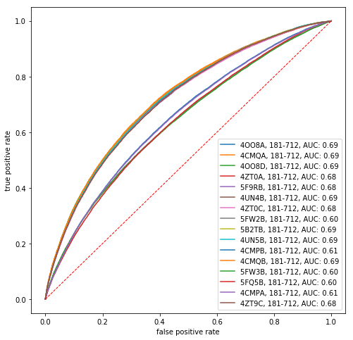
To further assess the extent to which direct information is predictive of protein contacts, we compute the receiver operating characteristic (ROC) curve that results from varying the number of predicted contacts. The ROC curve is the true positive rate, i.e. the number of correctly predicted contacts divided by the total number of contacts, versus the false positive rate, i.e. the number of incorrectly predicted contacts divided by the total number of noncontacting residue pairs. A perfect binary classifier has an area under the ROC curve equal to 1.

def roc(x, c):
    mask = np.triu(np.ones(di.shape[0], dtype=bool), k=2)
    order = x[mask].argsort()[::-1]
    c_flat = c[mask][order]
    tp = np.cumsum(c_flat, dtype=float)
    fp = np.cumsum(~c_flat, dtype=float)
    tp /= tp[-1]
    fp /= fp[-1]
    return fp, tp

fig, ax = plt.subplots(1, 1, figsize=(8, 8))
for i in range(refs.shape[0]):
    ref = refs.iloc[i]
    seq = msa[:, ref.seq]
    missing_aa_seq = seq == '-'
    di_idx = np.arange((~conserved_residues).sum())
    di_idx = di_idx[~missing_aa_seq[~conserved_residues]]
    di = direct_info[np.ix_(di_idx, di_idx)]
    contacts = contact_map(ref)
    fp, tp = roc(di, contacts)
    auc = tp.sum() / tp.shape[0]
    ax.plot(fp, tp, label='%s%s, %i-%i, AUC: %.02f' % (ref.pdb_id, ref.chain, ref.pdb_start, ref.pdb_end, auc))

grid = np.linspace(0, 1)
ax.plot(grid, grid, 'r--', lw=1)
ax.set_xlabel('false positive rate')
ax.set_ylabel('true positive rate')
plt.legend()
plt.show()

Structure exists: '../../../data/msa/Pfam-A.full/PF16592/pdb4oo8.ent'
Structure exists: '../../../data/msa/Pfam-A.full/PF16592/pdb4cmq.ent'
Structure exists: '../../../data/msa/Pfam-A.full/PF16592/pdb4oo8.ent'
Structure exists: '../../../data/msa/Pfam-A.full/PF16592/pdb4zt0.ent'
Structure exists: '../../../data/msa/Pfam-A.full/PF16592/pdb5f9r.ent'
Structure exists: '../../../data/msa/Pfam-A.full/PF16592/pdb4un4.ent'
Structure exists: '../../../data/msa/Pfam-A.full/PF16592/pdb4zt0.ent'
Structure exists: '../../../data/msa/Pfam-A.full/PF16592/pdb5fw2.ent'
Structure exists: '../../../data/msa/Pfam-A.full/PF16592/pdb5b2t.ent'
Structure exists: '../../../data/msa/Pfam-A.full/PF16592/pdb4un5.ent'
Structure exists: '../../../data/msa/Pfam-A.full/PF16592/pdb4cmp.ent'
Structure exists: '../../../data/msa/Pfam-A.full/PF16592/pdb4cmq.ent'
Structure exists: '../../../data/msa/Pfam-A.full/PF16592/pdb5fw3.ent'
Structure exists: '../../../data/msa/Pfam-A.full/PF16592/pdb5fq5.ent'
Structure exists: '../../../data/msa/Pfam-A.full/PF16592/pdb4cmp.ent'
Structure exists: '../../../data/msa/Pfam-A.full/PF16592/pdb4zt9.ent'