linear regression with conjugate gradient and a c++ matrix class

C++ is fast for scientific computing but has a cumbersome syntax. To make matrix computations easier to code, I wrote a templated matrix class in this repo. The class allows the programmer to define a matrix with matrix<double> A(3,3); and multiply two matrices with A*B, for example. To demonstrate the usefulness of the class, let’s solve the following linear regression problem:

Find the hyperplane $f(x)=c_0+c_1x_1+\cdots+c_nx_n$ that best fits the $m$ vectors $x^{(1)},\ldots,x^{(m)}\in\mathbb{R}^n$ and corresponding values $y_1,\ldots,y_m\in\mathbb{R}$, $m\gg n$; that is, find $c_0,c_1,\ldots,c_n\in\mathbb{R}$ that minimize the error $E=\sum_{i=1}^m [y_i-f(x^{(i)})]^2$.

Let’s first frame the problem in linear algebra. Write the vectors $x^{(i)}$ as the rows of a matrix $X$ with a prepended column of $1$s and arrange the coefficients $c_i$ in a vector $c$: \begin{align} X = \begin{pmatrix} 1 & x^{(1)}_1 & \cdots & x^{(1)}_n \\ 1 & x^{(2)}_1 & \cdots & x^{(2)}_n \\ \vdots & \vdots & & \vdots \\ 1 & x^{(m)}_1 & \cdots & x^{(m)}_n \end{pmatrix} \text{ and } c = \begin{pmatrix} c_0 \\ c_1 \\ \vdots \\ c_n \end{pmatrix}. \end{align}

Check for yourself that $E=\|y-Xc\|_2^2$ . To find the minimizer $c$, we will use conjugate gradient, an iterative method for solving $Ac=b$ for $c$ when $A$ is symmetric and positive definite. The method works by descending the quadratic energy function $\frac12x^TAx-x^Tb$ to its unique minimum in a sequence of directions $p_k$ conjugate with respect to $A$, i.e. $p_k^TAp_{k+1}=0$. The method is summarized by the following algorithm:

\begin{algorithm}
\caption{conjugate gradient}
\begin{algorithmic}
\PROCEDURE{cg}{$A, b, c_0, \varepsilon$}
\STATE $k = 0$
\STATE $p_0 = r_0 = b - Ac_0$
\WHILE {$\|r_k\|>\varepsilon$}
\STATE $\alpha_k = {r_k^Tr_k \over p_k^TAp_k}$
\STATE $c_{k+1} = c_k + \alpha_kp_k$
\STATE $r_{k+1} = r_k - \alpha_kAp_k$
\STATE $\beta_k = {r_{k+1}^Tr_{k+1} \over r_k^Tr_k}$
\STATE $p_{k+1} = r_{k+1} + \beta_kp_k$
\STATE $k = k+1$
\ENDWHILE
\RETURN $c_k$
\ENDPROCEDURE
\end{algorithmic}
\end{algorithm}

To see how this method is applicable to the linear regression problem, notice:

The image of $X$ at the minimizer $c$ is perpendicular to the residual $y-Xc$, so $X^T(y-Xc)=0$, and therefore the solution $c$ to $X^TXc=X^Ty$ minimizes $E$.
$X^TX$ is symmetric since it equals its transpose.
If $X$ has full rank i.e. if at least $n+1$ of the $x^{(i)}$ are independent, then $Xc\neq0$ for all $c\neq0$ and $c^TX^TXc=\|Xc\|_2^2>0$ for all $c\neq0$. That is, $X^TX$ is positive definite.

Then, let $A=X^TX$ and $b=X^Ty$. We will use the conjugate gradient method to solve $Ac=b$ for $c$. A conjugate gradient function using the matrix class in the matrix.hpp repo amounts to:

1
2
3
4
5
6
7
8
9
10
11
12
13
14
15
16
17
18
19
20
21
template <typename T>
matrix<T> conjugate_gradient(matrix<T> A, matrix<T> b, matrix<T> c0, T tol) {
  int k=0, n=A.shape[0]-1;
  matrix<T> c(n+1,1), p(n+1,1), r(n+1,1), Ap(n+1,1);
  T alpha, beta, rtr;

  p = r = b - A*c0;
  rtr = dot(r,r);
  while (norm(r) > tol) {
    Ap = A*p;
    alpha = rtr / dot(p, Ap);
    c = c + alpha*p;
    beta = rtr;
    r = r - alpha*Ap;
    rtr = dot(r,r);
    beta = rtr / beta;
    p = r + beta*p;
    k += 1;
  }
  return c;
}

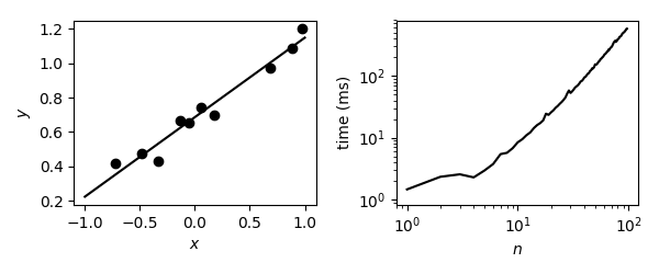
Here is a plot from $n=1$ and the execution time for $1\leq n<100$, with $m=10n$, $x^{(i)}_j\sim\mathcal{U}[-1,1]$, $y_i=f(x^{(i)})+\varepsilon$, and $\varepsilon\sim\mathcal{U}[-0.1,0.1]$.

linear regression results