Taylor’s Series
In order to compute the normal form of an equation \(\dot{x}=f(x)\), the normal_forms.normal_form.normal_form class first computes the Taylor series of \(f(x)\) up to a specified degree \(k\). The class that implements the Taylor series of \(f(x)\) at a specified center \(x_0\) up to a specified degree \(k\) is normal_forms.jet.jet.
The reason why the class is called jet is that the \(k\)-jet centered at \(x_0\) of a function \(f(x)\) is the Taylor’s series truncated at degree \(k\):
Like when creating a normal_form object, \(f(x)\), \(x_0\), and \(k\) should be supplied to create the jet object, and non-algebraic functions in \(f(x)\) should be defined with the sympy variants of those functions. Once the jet is created, it can be evaluated at points in the domain:
In [1]: from normal_forms import jet

In [2]: import sympy

In [3]: f = lambda x: sympy.exp(x)

In [4]: h = jet(f, x=0, k=10)

In [5]: h(1)
Out[5]: 2.718281801146385
The formula above makes sense for \(f:\mathbb{R}^n\rightarrow\mathbb{R}^p\) with any natural number dimensions \(n\) and \(p\) when \(m\) is a multiindex \(m=(m_1,\ldots,m_n)\) with derivative, exponent, factorial, and absolute value defined as
To follow are a few examples for different choices of domain \(\mathbb{R}^n\) and range \(\mathbb{R}^p\) of \(f\).
A \(\mathbb{R}\rightarrow\mathbb{R}\) example
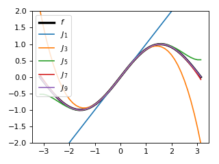
The domain and range may have the same dimension, for example, \(f(x)=\sin(x)\):
(Source code, png, hires.png, pdf)

A \(\mathbb{R}\rightarrow\mathbb{R}^2\) example
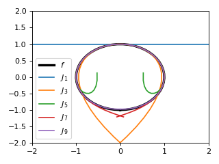
The dimension of the range may be greater than the dimension of the domain, for example, \(f(t)=(\sin(t),\cos(t))\) viewed here as a parametric plot in the \(xy\)-plane:
(Source code, png, hires.png, pdf)

A \(\mathbb{R}^2\rightarrow\mathbb{R}\) example
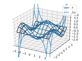
The dimension of the range may be less than the dimension of the domain, for example, \(f(x,y)=\sin(x)\cos(y)\):
(Source code, png, hires.png, pdf)
