derivatives of the sigmoid function
The sigmoid function $f(x)={1 \over 1+e^{-x}}$ is useful in a variety of applications particularly because it can be used to map an unbounded real value into $[0,1]$. As the solution to $y’=y(1-y)$, $y(0)=1/2$, it is used as the prototypical model of population growth with a carrying capacity. It can be used as a so-called activation function that compactifies inputs to nodes in a neural network. I used the function extensively in my own research to model the probability that an ion channel on an electrically excitable cell’s membrane opens in responses to a voltage change.
The sigmoid function is smooth, i.e. has infinitely many continuous derivatives. Just for kicks, I asked whether I could come up with a formula for the $n^{th}$ derivative $f^{(n)}$. I was able to, and the key observations to my approach were
-
$f^{(n)}$ can be written as a series with coefficients multiplying powers of $f$, and
-
${d\over dx}$ restricted to truncated series of this form can be written in a neat matrix form.
I don’t know if this proof is novel, but it surprised me how much linear algebra it involved, so I will share. Here’s the result:
derivative formula
The $n^{th}$ derivative of $f(x)={1 \over 1+e^{-x}}$ is
proof
First, notice that $f’$ is the quadratic series $f-f^2$:
Since $f(x)=(1+e^{-x})^{-1}$, by the chain rule $f’(x)=(1+e^{-x})^{-2}e^{-x}$. With some algebra and noticing $1-f(x)={e^{-x} \over 1+e^{-x}}$, we have $f’(x)={1 \over 1+e^{-x}}{e^{-x} \over 1+e^{-x}} = f(x)[1-f(x)]$.
Next, by the chain rule $(f^k)’=kf^{k-1}f’=kf^k-kf^{k+1}$.
That is to say any term $c_kf^k$ in a series of the form $\sum_{k=1}^{\infty}c_kf^k$ gets mapped by ${d \over dx}$ to $c_kkf^k-c_kkf^{k+1}$. Since $f$ itself is obviously a series of this form ($c_1=1$, $c_k=0$ for $k>1$), hopefully you can imagine differentiating $f$ repeatedly and collecting the powers of $f$ at each step. Linear algebra will help us do this systematically.
Let’s represent truncated series of the form $\sum_{k=1}^{n}c_kf^k$ by vectors of their coefficients $c=\begin{pmatrix}c_1&\cdots &c_n&0\end{pmatrix}^T$. The extra zero is to make room for the $(n+1)^{st}$ power of $f$ that will result from differentiation. The derivative of the truncated series is represented by $D_{n}c$ with the differentiation operator written as the matrix
That column $k$ of $D_{n}$ has $k$ on the diagonal and $-k$ on the subdiagonal ensures that the $k^{th}$ coordinate of $c$ contributes $kc_k$ and $-kc_k$ to the $k^{th}$ and $(k+1)^{st}$ coordinates of the product. This is what we should expect from the above remarks on $(c_kf^k)’$.
Here’s the leap. $D_{n}$ has $n+1$ distinct eigenvectors
with corresponding eigenvalues $j+1$, with the convention ${i\choose j}=0$ if $i<j$. I’ll defer the proof of this claim to after the current proof. Now, we realize the utility of eigendecompositions for powering.
The sigmoid function $f$ is represented by the alternating sum of the eigenvectors
Sum across the rows of Pascal’s triangle with alternating terms to convince yourself of this last claim:
\begin{array}{ccccc}
+v_{n,0} & -v_{n,1} & +v_{n,2} & -v_{n,3} & \cdots & (-1)^nv_{n,n} \\
1 & -0 & 0 & -0 & & 0 \\
1 & -1 & 0 & -0 & & 0 \\
1 & -2 & 1 & -0 & & 0 \\
1 & -3 & 3 & -1 & & 0 \\
\vdots & & & & \ddots & \vdots \\
{n\choose0} & -{n\choose1} & {n\choose2} & -{n\choose3} & \cdots & (-1)^n{n\choose n}
\end{array}
The work of repeatedly differentiating $f$ is done by repeatedly multiplying its vector of coefficients by $D_n$. The $n^{th}$ derivative of $f$ is represented by $D_n^n\begin{pmatrix}1&0&\cdots&0\end{pmatrix}^T$:
\begin{aligned}
D_n^n\sum_{j=0}^n(-1)^jv_{n,j} &= \sum_{j=0}^n(-1)^jD_n^nv_{n,j} \\
&= \sum_{j=0}^n(-1)^j(j+1)^nv_{n,j}.
\end{aligned}
The $k^{th}$ coordinate of this vector is $\sum_{j=0}^n(-1)^j(j+1)^n{k-1 \choose j}$.
Coming back from vector representations to series of the form $\sum_{k=1}^{\infty}c_kf^k(x)$, that last expression is a formula for the coefficient $c_k$ of $f^{(n)}$ as such a series. Then, the full series is $\sum_{k=1}^{\infty}\sum_{j=0}^{\infty}(-1)^j(j+1)^n{k-1 \choose j}f^k(x)$.
The series gains only one new power of $f$ each time differentiation is applied ($D_n$ is nonzero on the subdiagonal but 0 below the subdiagonal) so we can truncate the $k$ index of the series corresponding to $f^{(n)}$ at $n+1$, and with the convention of the binomial coefficient (“choose”) operator mentioned above, we can truncate the $j$ index of that series at $k-1$, so Finally, we shift the $k$ index to start at $0$ to obtain the exact statement of the result above.
deferred proof
eigenpairs of $D_n$
We will show by induction that $D_n$ has eigenvectors $v_{n,j}$, $j=0,\ldots,n$, with eigenvalues $j+1$.
The $n=0$ base case is to confirm that the scalar $1$ has an eigenvector $1$ with eigenvalue $1$, which is obvious.
For the induction step, assume for $k>0$ that $D_{k-1}$ has eigenvectors $v_{k-1,j}$, $j=0,\ldots,k-1$, with eigenvalues $j+1$.
We have
\begin{aligned}
D_kv_{k,j} &=
\begin{pmatrix} D_{k-1} & 0 \\ \begin{pmatrix} 0 & \cdots & 0 & -k \end{pmatrix} & k+1 \end{pmatrix}
\begin{pmatrix} v_{k-1,j} \\ {k\choose j} \end{pmatrix} \\
&= \begin{pmatrix} D_{k-1}v_{k-1,j} \\ -k{k-1\choose j}+(k+1){k\choose j} \end{pmatrix}.
\end{aligned}
The top of this block vector is $(j+1)v_{k-1,j}$ by the induction step, and the first term of the bottom can be rearranged
\begin{aligned}
-k{k-1\choose j} &= -{k(k-1)! \over j!(k-j-1)!} \\
&= -(k-j){k!\over j!(k-j)!} \\
&= (j-k){k\choose j}
\end{aligned}
so that the bottom is $(j+1){k\choose j}$. Thus, $D_kv_{k,j}=(j+1)v_{k,j}$.
plots
Here’s a plot of the derivatives of the sigmoid function using the above formula:
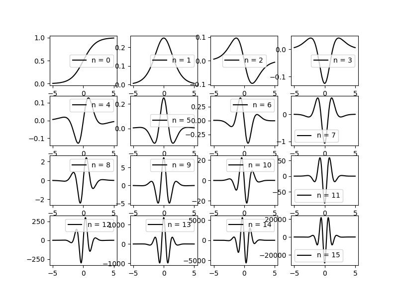
And, here’s the Python script that produced the plot:
import numpy as np
import matplotlib.pyplot as plt


def f(x):
    """sigmoid function"""
    return 1.0 / (1.0 + np.exp(-x))


def df(n, x):
    """nth derivative of sigmoid function"""
    # compute coeffs
    c = np.zeros(n + 1, dtype=int)
    c[0] = 1
    for i in range(1, n + 1):
        for j in range(i, -1, -1):
            c[j] = -j * c[j - 1] + (j + 1) * c[j]
    # compute derivative as series
    res = 0.0
    for i in range(n, -1, -1):
        res = f(x) * (c[i] + res)
    return res


x = np.linspace(-5, 5, 1000)[:, np.newaxis].repeat(16, axis=1).T
y = np.array([df(n, x[n]) for n in range(16)])

fig, ax = plt.subplots(4, 4, figsize=(8, 6))
for xi, yi, i in zip(x, y, range(16)):
    ax[i / 4, i % 4].plot(xi, yi, 'k-', label="n = %i" % (i))
    ax[i / 4, i % 4].legend()
plt.savefig('../assets/img/sigmoid-derivs.png')
Note this implementation becomes unstable at about $n=20$ because the terms in the above formula are alternating and grow rapidly in magnitude with $n$.